This document is intended to assist those who want to know exactly how many classes all of your students have missed at the end of a term…something Roll Call will not do for you on its own. This is especially problematic for instructors who (for example) start deducting points once students have missed X number of classes, but do not necessarily base a grade on the total number of absences a student has.
One of the questions that I will often get from instructors at the end of the term is how to tell exactly how many (and when) students were absent/late for a specific class. While I realize this document will go out of date the very second the Roll Call Attendance feature gets fully revamped, I want to at least show the steps that instructors can take who need the numbers that the Roll Call report provides....especially for those who have never opened a CSV file before, much less tried creating a pivot table in Excel. Please note this guide uses screen captures from a Windows 7-based PC, using Excel 2013.
For those folks who do not have Excel AT ALL, are on Macs, or just want a really, really simple solution, I invite you check out my other online document, https://community.canvaslms.com/docs/DOC-12524-easy-to-use-google-sheet-for-interpreting-your-roll-c... . The only prerequisite for that is having a Google Drive account and knowing how to copy/paste. Otherwise, virtually everything else is done for you. Really.
The Quick and Dirty Method
While the Attendance column in the Gradebook will let you know the percentage of times a student was present (or the point value, if you adjusted this default setting) many people do not realize that a simple count is available right back under the Attendance menu item. If you head there, simply click on the MORE link next to any given student's name, and that will tell you exactly the number of times a student was present, absent, or late:

This "trick" will always show the TOTAL number for all dates thus far when attendance was taken; you do not necessarily have to be on today's date to show the grand total for the term, since it always will. While this method is fine for smaller classes, it is obviously a major pain if you want a quick count of the number of times each student was absent in much larger classes. Enter the Roll Call report....
Dealing With a CSV File....Even if You Loathe Excel
Okay; on to the dreaded CSV file, which this guide hopes to make a bit easier those of you not terribly Excel-savvy. If you follow the instructions for running a Roll Call report, you will have a roll call report link emailed to you. (No, it is not instantaneously done online, but the email and accompanying link—which is good for only 24 hours—is emailed very quickly.) For an entire class report, do not put in the student ID number on the form you submit to Canvas, just the start date and end date for your course.
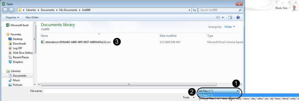
Once you have clicked the link and saved the CSV file, you can open it in Excel. For most users, just double-clicking on a CSV file will open Excel automatically. If for some reason that does not work, open Excel first and navigate your way to where you saved the CSV file, and then make sure that Excel will recognize ALL file types. You should then find the CSV file in the directory where you saved it:

Once you've opened it, do a quick FILE>>SAVE AS and make sure you save the CSV file as an Excel file.
Deleting Some Columns and Getting Ready to Create a Pivot Table
When you open the file, it will look a bit like this:

The top row--number 1--shows the column heading names, while everything underneath is the data itself. Fortunately, you do not need all of those columns to create the pivot tables that you likely need to create a listing of classes each student missed. In fact, I recommend removing the first SEVEN columns: Course ID, SIS Course ID, Course Code, Course Name, Teacher ID, Teacher Name. Why can the course information be deleted? Because for one thing, the CSV file is for just one course, not all of your courses. And even if you teach a multi-sectioned course that has been combined into one Canvas course site, the CSV file contains ALL sections in one file. (Hurrah!)
The teacher information can also be removed, since you likely already know your own name(!) But seriously, if you share teaching duties with others in a multi-sectioned course site, you may have to keep those columns. (Maybe try doing that after you have learned a few pivot table basics, outlined below.) But for this example, we will delete those columns because we are dealing with just one instructor.
I would argue you can even remove the Student ID column. Unless you have students with the EXACT same name, that can safely be deleted. We will leave it for this example, since some of you may have that very issue in larger classes, but for you instructors in smaller institutions you can likely dump that column, as well.
Removing columns in Excel is very easy. Taking that big, plus-sign shaped Excel cursor, and just click and drag anywhere within the spreadsheet across the columns you wish to remove. It can even be just one row. What you select will appear highlighted. Then, while they are highlighted, on the HOME tab click the Delete button, and click Delete Sheet Columns. This whole procedure will look something like this:

Presto! You are now down to far fewer columns. Finally, delete the Timestamp column the same way. (All that column does is record when you took attendance, which you do not need to know. The valuable Class Date and Attendance columns in the spreadsheet are the ones that keep track of the attendance data that you laboriously took all term.)
For those of you who have never ventured into Excel at all before, you can widen the columns in your spreadsheet by hovering your mouse between the lettered column headings until you see a double-sided arrow icon, and then click and drag the columns to make them a bit wider. (See below, which also shows what your spreadsheet should be looking like about now):

This step is NOT absolutely necessary, though I realize many people like to see all of the data they are about to work with! We are now ready to create the first of two (possibly) pivot tables, depending on your needs.
Pivot Table Number 1: Number of times Present/Absent
Your first pivot table will pretty much replicate what you would get by clicking on that MORE button outlined at the beginning of this document: an alphabetical listing of all students (by first name, alas…that's how it's exported) and the number of classes for which they were present/absent/late (assuming you tracked the latter).
Step One: Select Your Data
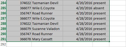
Excel needs to know exact the data you want to create a pivot table from, so you first task is selecting all data in your spreadsheet. Fortunately, you do not have to click-and-drag through hundreds of rows to do this! Without getting too caught up in technicalities, just make sure your mouse is in the top-most cell: A1, the Student ID cell. Then, simply press Ctrl-A on your keyboard. Voila! Everything in the first four columns is selected, but nothing after it:

Step Two: Insert a Pivot Table
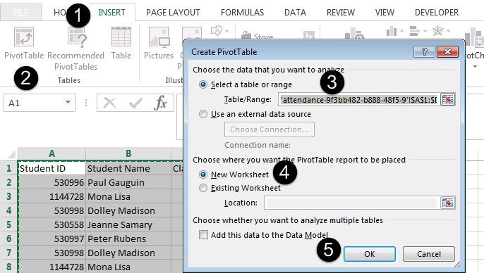
Now, with that data selected, head to the top and click the INSERT tab, and then select Pivot Table. (Trust me: Recommended Pivot Tables is not going to do you a lick of good for this.) You will then see a dialog box. Your selection should already be populated in the top-most text box for Select a table or range. Then, make sure that the New Worksheet radio button is selected:

You will now be on a newly-created worksheet (Sheet1) staring at a Pivot Table Fields dialog box. We are going to keep things simple here. On the top part of the dialog box, select all of the fields. (Though again, Student ID is optional for most. Unless you really, really need the Student ID number, do NOT check that box.) The dialog box will look something like this:

Step Three: Adjust the Pivot Table Fields
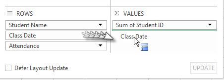
You will already see the results of your pivot table on your spreadsheet, but we are not finished. Next, click-and-drag the Class Date field over to the column on the right (Values). If you included the Student ID field, it will likely be there, as well. If you did not include the Student ID file, that's fine…but still click-and-drag Class Date over to that area:

(In the unlikely event that the Attendance field is listed above Student Name in the left area, click the drop-down menu next to Student Name and select Move Up. We want Student Name first, and then Attendance in that left column after moving over Class Date to the right.)
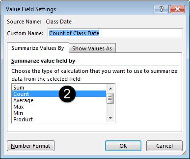
The newly-added field should say Count of Class Date. If it does not, click the drop-down menu for it and select the last choice: Value Field Settings. On the ensuing dialog box, enable Count and click OK, as shown below:


You are probably seeing by now why that Student ID data field can be kind of a pain if you left it there. By default, Excel is likely summing it. If you really DID need that Student ID field to differentiate one student from another, my suggestion is to click the drop-down menu for that field and select Value Field Settings and simply select Max. (Which technically will show the maximum student ID number for each student. Since each student has but one ID number, it effectively will show only the ID number.)
When this is all said and done, your pivot table will look like this. It is important the fields are in the order shown below in the Rows and Values column:

Congratulations! You have just created a pivot table in Excel that lists all of your students and the total number of days they were in class (or not). What you basically did was arrange everything by Student Name, sub-sorted by the Attendance status (Absent, Present, etc.). Then, Excel performed a COUNT of all of the Class Dates for each student in the Attendance column.
Pivot Table Number 2: Listing of Dates for Each Student and Attendance
That first pivot table is one we get requested for the most. This next one will take you through the same steps, only this time will list each student and a class date-by-class date listing.
To do this, do absolutely everything we did for the first pivot table: select the data, click INSERT>>PIVOT TABLE, and check off the fields that you need. The Pivot Table Fields dialog box will look exactly the same as the first one we did. Again, leave Student ID out if you can. If not, go ahead and include it.
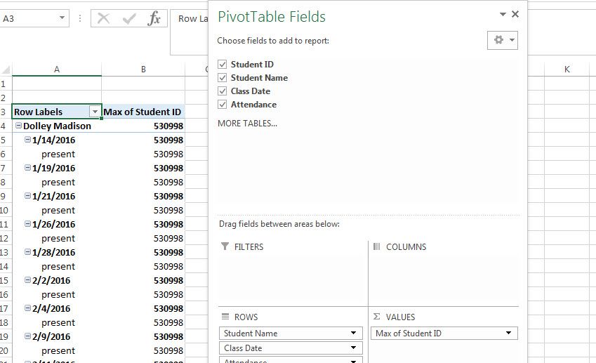
Believe it or not, that's it! You show now have a listing of each student and a chronological listing of the class dates underneath, plus whether the student was present or absent. This time, the Student ID number comes out just fine for each individual day, though if you're a perfectionist you can change the Student ID over on the right to Max as we did for the first example.
Your pivot table will look something like this. This capture also shows you how the fields (and in which columns) they should be listed to produce this result, so that you can make the proper adjustments:

I hope you find this overview useful. I know there are LOTS of other things you can do with pivot tables, and some of you may even object to the way I did certain things here, but I wanted to make this easy enough for everyone to understand--even those who do not use Excel. I welcome your comments and am happy to entertain any suggestions for improving things.

