Thank you for providing an idea of how students can do this with Excel, and the notation on the additional boxes. I looked closer after you shared this to see some of the weirdness in how it merges/doesn't merge cells. Weird. A CSV export option would be helpful for this.
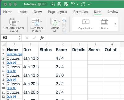
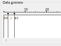
There is an easier way to get the Text to Columns to produce the desired outcome without having to use the Find & Replace tool. Highlight the original cell containing the score (for example, 4 / 4 in your the first assignment from your picture. When you go to the Text to Columns feature, instead of Delineator, choose Fixed Width and hit Next. On the next step, you will see a preview at the bottom with an arrow, most likely right after the slash. Drag that arrow over to the four and click right after the first value to add a second arrow. It should look like this:

This will split up the text into three columns, the first and last containing the values as numbers. Then just delete the middle column and change the headings as needed. When I tried to find a way to use Delineators, it kept outputting the first number with extra spaces, which then required modifying (or Find and Replace like you mentioned) in order to remove the space so it can be used in formulas without error. The Fixed Width option eliminates that issue.
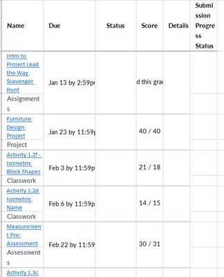
You would still need to delete the extra rows to help with calculations. BTW, only the score and date columns have merged cells. After importing, select every other row and just right click to get the delete rows option. It will "unmerge" the other cells at the same time. Yep, another step, but one that could quickly fix that issue for the calculating without having to unmerge first.
If you need the "type" of assignment (Assignment, Quiz, Discussion, etc) that is in the row under the title, there is another quick way to move that to another spot to preserve it for your category average goal. Here is a possible workflow:
- After copying the data, delete any columns you do not need (I deleted Status and Details, and base the steps below on that)
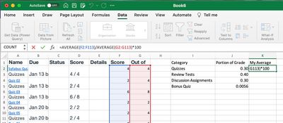
- Use Text to Columns, with the Fixed Width option described above, to split out the scores. Delete the column with the slash. Use =C2/D2 (or whatever your columns are) in E2 to get a percentage, then use the drag to fill to complete the calculations for the remaining rows.
- Go to F2. Type the following: =IF(ISODD(ROW(A3)),A3,"") - The A3 in this spot represents the cell that contains the category, assuming you pasted everything into A1 to start. Then use the drag to fill option and pull down to the last row. This will skip every other row in column F2.
- Select the alternating rows originally containing the assignment type and delete them.
This should get it set up for whatever remaining work you want students to do. I wish there was an quicker way, but maybe this will help to eliminate some steps while teaching showing students the power of Excel.
